In "Making Model Training More Scientific (Part 5): Fine-tuning Learning Rates Based on Gradients", we entered a new chapter on scheduling learning rates based on gradients. However, it was mentioned at the end of the previous article that when deriving the optimal learning rate for terminal loss under dynamic gradients, we encountered difficulties in the proof. Specifically, it is extremely difficult to verify the optimal learning rate sequence "guessed" via variational methods by substituting it into the conclusion for scaling. Consequently, we couldn't even determine if the sequence was a feasible solution, let alone the optimal one.
In this article, we will obtain a more precise conclusion through an exquisite construction, thereby solving this problem. Judging by the proof process, the precision of this conclusion may have reached a point where it can no longer be improved. This breakthrough also originates from the paper "Optimal Linear Decay Learning Rate Schedules and Further Refinements".
Problem Review #
Let's first review the previous conclusions. At the end of the last post, we obtained a general version of the conclusion from "Making Model Training More Scientific (Part 4): New Identity, New Learning Rate": \begin{equation}\mathbb{E}[L(\boldsymbol{\theta}_T) - L(\boldsymbol{\theta}^*)] \leq \frac{R^2}{2\eta_{1:T}} + \frac{1}{2}\sum_{t=1}^T\frac{\eta_t^2 G_t^2}{\eta_{\min(t+1, T):T}}\label{leq:last-2}\end{equation} We want to find a sequence $\eta_1,\eta_2,\cdots,\eta_T\geq 0$ that minimizes the right-hand side of the above inequality. Through continuous approximation and variational methods, we "guessed" the answer to be: \begin{equation}\eta_t = \frac{R G_t^{-2}}{\sqrt{Q_T}} (1 - Q_t/Q_T)\label{eq:opt-lr-last-x}\end{equation} where $Q_t=\sum_{k=1}^t G_k^{-2}$. However, we couldn't prove it by direct substitution; or rather, proving it requires additional assumptions. If we try to substitute it, we find the main issue is that the denominator on the right side of Eq. $\eqref{leq:last-2}$ is $\eta_{t+1:T}$ (when $t < T$), making it impossible to guarantee that $\eta_t/\eta_{t+1:T}$ is bounded, which makes various scalings very difficult. If we can further improve the denominator on the right side of the conclusion to $\eta_{t:T}$, the proof will follow naturally.
This article achieves the final proof by further improving the precision of conclusion $\eqref{leq:last-2}$, but not by improving it directly and explicitly. Instead, through careful scaling, it constructs the optimal learning rate sequence from the top down, achieving the effect of implicitly improving precision.
Careful Scaling #
Specifically, our starting point is the identity from "Making Model Training More Scientific (Part 4): New Identity, New Learning Rate": \begin{equation}\begin{aligned} q_T =&\, \frac{1}{w_{1:T}}\sum_{t=1}^T w_t q_t + \sum_{k=1}^{T-1}\left(\frac{1}{w_{k+1:T}} - \frac{1}{w_{k:T}}\right)\sum_{t=k}^T w_t (q_t - q_k) \\ =&\, \frac{1}{w_{1:T}}\sum_{t=1}^T w_t q_t + \sum_{k=1}^{T-1}\left(\frac{1}{w_{k+1:T}} - \frac{1}{w_{k:T}}\right)\sum_{t=k+1}^T w_t (q_t - q_k) \end{aligned}\label{eq:qt-g}\end{equation} Let $q_t = \mathbb{E}[L(\boldsymbol{\theta}_t) - L(\boldsymbol{\theta}^*)]$, where $\mathbb{E}$ is the expectation over all $\boldsymbol{x}_1, \boldsymbol{x}_2, \cdots, \boldsymbol{x}_T$. Substituting this into the above formula gives: \begin{equation}\mathbb{E}[L(\boldsymbol{\theta}_T) - L(\boldsymbol{\theta}^*)] = \frac{1}{w_{1:T}}\sum_{t=1}^T w_t \mathbb{E}[L(\boldsymbol{\theta}_t) - L(\boldsymbol{\theta}^*)] + \sum_{k=1}^{T-1}\left(\frac{1}{w_{k+1:T}} - \frac{1}{w_{k:T}}\right)\sum_{t=k+1}^T w_t \mathbb{E}[L(\boldsymbol{\theta}_t) - L(\boldsymbol{\theta}_k)]\label{eq:qt-g2}\end{equation} From now on, we must adhere to the principle of "no scaling unless necessary" to achieve the highest possible precision. Now we use convexity for the first scaling: \begin{gather} \mathbb{E}[L(\boldsymbol{\theta}_t) - L(\boldsymbol{\theta}^*)] = \mathbb{E}[L(\boldsymbol{x}_t, \boldsymbol{\theta}_t) - L(\boldsymbol{x}_t, \boldsymbol{\theta}^*)] \leq \mathbb{E}[\boldsymbol{g}(\boldsymbol{x}_t, \boldsymbol{\theta}_t)\cdot(\boldsymbol{\theta}_t - \boldsymbol{\theta}^*)] \\[4pt] \mathbb{E}[L(\boldsymbol{\theta}_t) - L(\boldsymbol{\theta}_k)] = \mathbb{E}[L(\boldsymbol{x}_t, \boldsymbol{\theta}_t) - L(\boldsymbol{x}_t, \boldsymbol{\theta}_k)] \leq \mathbb{E}[\boldsymbol{g}(\boldsymbol{x}_t, \boldsymbol{\theta}_t)\cdot(\boldsymbol{\theta}_t - \boldsymbol{\theta}_k)] \end{gather} Note that this requires each $\boldsymbol{\theta}_t$ to depend at most on $\boldsymbol{x}_1, \boldsymbol{x}_2, \cdots, \boldsymbol{x}_{t-1}$, which is satisfied in stochastic optimization. Furthermore, the first equality in the second line requires $t \geq k$, which is also obviously satisfied. Substituting into Eq. $\eqref{eq:qt-g2}$ yields: \begin{equation}\mathbb{E}[L(\boldsymbol{\theta}_T) - L(\boldsymbol{\theta}^*)] \leq \underbrace{\frac{1}{w_{1:T}}\sum_{t=1}^T w_t \mathbb{E}[\boldsymbol{g}(\boldsymbol{x}_t, \boldsymbol{\theta}_t)\cdot(\boldsymbol{\theta}_t - \boldsymbol{\theta}^*)]}_{(\text{A})} + \underbrace{\sum_{k=1}^{T-1}\left(\frac{1}{w_{k+1:T}} - \frac{1}{w_{k:T}}\right)\sum_{t=k+1}^T w_t \mathbb{E}[\boldsymbol{g}(\boldsymbol{x}_t, \boldsymbol{\theta}_t)\cdot(\boldsymbol{\theta}_t - \boldsymbol{\theta}_k)]}_{(\text{B})}\label{leq:last-6-mid}\end{equation} In the article "Making Model Training More Scientific (Part 4): New Identity, New Learning Rate", the next step was to scale $(\text{A})$ and $(\text{B})$ in Eq. $\eqref{leq:last-6-mid}$ separately and then add them. This separate processing magnified the errors and created trouble for the subsequent proof.
Identical Transformation #
Therefore, in this section, we will merge them into a single expression through mathematical identities before considering scaling, to achieve higher precision. First, still assuming the learning rate is independent of data $\boldsymbol{x}_t$, we can pull the expectation $\mathbb{E}$ outside: \begin{equation}\mathbb{E}[L(\boldsymbol{\theta}_T) - L(\boldsymbol{\theta}^*)] \leq \mathbb{E}\Bigg[\underbrace{\frac{1}{w_{1:T}}\sum_{t=1}^T w_t \boldsymbol{g}(\boldsymbol{x}_t, \boldsymbol{\theta}_t)\cdot(\boldsymbol{\theta}_t - \boldsymbol{\theta}^*)}_{(\text{A})} + \underbrace{\sum_{k=1}^{T-1}\left(\frac{1}{w_{k+1:T}} - \frac{1}{w_{k:T}}\right)\sum_{t=k+1}^T w_t \boldsymbol{g}(\boldsymbol{x}_t, \boldsymbol{\theta}_t)\cdot(\boldsymbol{\theta}_t - \boldsymbol{\theta}_k)}_{(\text{B})}\Bigg]\end{equation} The second term is more complex. Swapping the summation order using $\sum_{k=1}^{T-1}\sum_{t=k+1}^T = \sum_{t=1}^T \sum_{k=1}^{t-1}$: \begin{equation}\begin{aligned} (\text{B}) =&\, \sum_{t=1}^T \sum_{k=1}^{t-1}\left(\frac{1}{w_{k+1:T}} - \frac{1}{w_{k:T}}\right) w_t \boldsymbol{g}(\boldsymbol{x}_t, \boldsymbol{\theta}_t)\cdot(\boldsymbol{\theta}_t - \boldsymbol{\theta}_k) \\ =&\, \sum_{t=1}^T w_t \boldsymbol{g}(\boldsymbol{x}_t, \boldsymbol{\theta}_t)\cdot \sum_{k=1}^{t-1}\left(\frac{1}{w_{k+1:T}} - \frac{1}{w_{k:T}}\right) (\boldsymbol{\theta}_t - \boldsymbol{\theta}_k) \\ =&\, \sum_{t=1}^T w_t \boldsymbol{g}(\boldsymbol{x}_t, \boldsymbol{\theta}_t)\cdot \left(\left(\frac{1}{w_{t:T}} - \frac{1}{w_{1:T}}\right)\boldsymbol{\theta}_t - \sum_{k=1}^{t-1}\left(\frac{1}{w_{k+1:T}} - \frac{1}{w_{k:T}}\right) \boldsymbol{\theta}_k\right) \\ \end{aligned}\end{equation} Adding $(\text{A})$, the term $\frac{1}{w_{1:T}}w_t \boldsymbol{g}(\boldsymbol{x}_t, \boldsymbol{\theta}_t)\cdot\boldsymbol{\theta}_t$ is exactly cancelled. Organizing the rest: \begin{equation}\mathbb{E}[L(\boldsymbol{\theta}_T) - L(\boldsymbol{\theta}^*)] \leq \mathbb{E}\Bigg[\frac{1}{w_{1:T}}\sum_{t=1}^T w_t \boldsymbol{g}(\boldsymbol{x}_t, \boldsymbol{\theta}_t)\cdot\Bigg(\underbrace{\frac{w_{1:T}}{w_{t:T}}\boldsymbol{\theta}_t - w_{1:T}\sum_{k=1}^{t-1}\left(\frac{1}{w_{k+1:T}} - \frac{1}{w_{k:T}}\right) \boldsymbol{\theta}_k}_{\text{denoted as }\boldsymbol{\psi}_t} - \boldsymbol{\theta}^*\Bigg)\Bigg]\end{equation} As long as we denote the indicated part above as $\boldsymbol{\psi}_t$, the right-hand side takes the standard form of (weighted) average loss convergence: \begin{equation}\mathbb{E}[L(\boldsymbol{\theta}_T) - L(\boldsymbol{\theta}^*)] \leq \mathbb{E}\Bigg[\frac{1}{w_{1:T}}\sum_{t=1}^T w_t \boldsymbol{g}(\boldsymbol{x}_t, \boldsymbol{\theta}_t)\cdot(\boldsymbol{\psi}_t - \boldsymbol{\theta}^*)\Bigg] = \frac{1}{w_{1:T}}\sum_{t=1}^T w_t \mathbb{E}[\boldsymbol{g}(\boldsymbol{x}_t, \boldsymbol{\theta}_t)\cdot(\boldsymbol{\psi}_t - \boldsymbol{\theta}^*)]\label{leq:last-6-mid2}\end{equation}
Update Rules #
According to the definition of $\boldsymbol{\psi}_t$, it can be directly verified that: \begin{equation}\boldsymbol{\psi}_{t+1} - \boldsymbol{\psi}_t = \frac{w_{1:T}}{w_{t+1:T}}(\boldsymbol{\theta}_{t+1} - \boldsymbol{\theta}_t)\end{equation} Therefore, if we let $\boldsymbol{\psi}_t$ update according to $\boldsymbol{\psi}_{t+1} = \boldsymbol{\psi}_t - w_t \boldsymbol{g}(\boldsymbol{x}_t, \boldsymbol{\theta}_t)$, then we will have $\boldsymbol{\theta}_{t+1} = \boldsymbol{\theta}_t - \frac{w_t w_{t+1:T}}{w_{1:T}} \boldsymbol{g}(\boldsymbol{x}_t, \boldsymbol{\theta}_t)$: \begin{equation}\boldsymbol{\psi}_{t+1} = \boldsymbol{\psi}_t - w_t \boldsymbol{g}(\boldsymbol{x}_t, \boldsymbol{\theta}_t)\qquad\Rightarrow\qquad\boldsymbol{\theta}_{t+1} = \boldsymbol{\theta}_t - \frac{w_t w_{t+1:T}}{w_{1:T}} \boldsymbol{g}(\boldsymbol{x}_t, \boldsymbol{\theta}_t)\end{equation} For $\boldsymbol{\psi}_t$ following this update rule, we have already proved in "Making Model Training More Scientific (Part 2): Extending Conclusions to Unbounded Domains" and "Making Model Training More Scientific (Part 5): Fine-tuning Learning Rates Based on Gradients" that the following inequality holds: \begin{equation}\frac{1}{w_{1:T}}\sum_{t=1}^T w_t \mathbb{E}[\boldsymbol{g}(\boldsymbol{x}_t, \boldsymbol{\theta}_t)\cdot(\boldsymbol{\psi}_t - \boldsymbol{\theta}^*)] \leq \frac{1}{2 w_{1:T}}\left(R^2 + \sum_{t=1}^T w_t^2 \mathbb{E}[\Vert\boldsymbol{g}(\boldsymbol{x}_t, \boldsymbol{\theta}_t)\Vert^2]\right)\label{leq:avg-3}\end{equation} where $R = \Vert\boldsymbol{\psi}_1 - \boldsymbol{\theta}^*\Vert$. If we choose the same starting point for $\boldsymbol{\psi}_t$ and $\boldsymbol{\theta}_t$, then we also have $R = \Vert\boldsymbol{\theta}_1 - \boldsymbol{\theta}^*\Vert$.
Readers might find something amiss: the $\boldsymbol{g}(\boldsymbol{x}_t, \boldsymbol{\theta}_t)$ in the above formula is the gradient at $\boldsymbol{\theta}_t$ rather than at $\boldsymbol{\psi}_t$. Can it still be substituted into the previous conclusion? Regarding this, we specifically clarified in "Part 5" that the role of using the gradient at the current point $\boldsymbol{g}(\boldsymbol{x}_t, \boldsymbol{\psi}_t)$ is to establish the relationship between $\boldsymbol{g}(\boldsymbol{x}_t, \boldsymbol{\psi}_t)\cdot(\boldsymbol{\psi}_t - \boldsymbol{\theta}^*)$ and the loss function through convexity. But since we do not need that relationship here, replacing it with $\boldsymbol{g}(\boldsymbol{x}_t, \boldsymbol{\theta}_t)$ is acceptable.
Strongest Conclusion #
Now, substituting conclusion $\eqref{leq:avg-3}$ into Eq. $\eqref{leq:last-6-mid2}$ and performing the second scaling, we get: \begin{equation}\mathbb{E}[L(\boldsymbol{\theta}_T) - L(\boldsymbol{\theta}^*)] \leq \frac{1}{2 w_{1:T}}\left(R^2 + \sum_{t=1}^T w_t^2 G_t^2\right)\label{leq:last-6}\end{equation} Here we denote $G_t^2 = \mathbb{E}[\Vert\boldsymbol{g}(\boldsymbol{x}_t, \boldsymbol{\theta}_t)\Vert^2]$. That is to say, if we perform SGD with a learning rate $\eta_t = \frac{w_t w_{t+1:T}}{w_{1:T}}$, its final loss satisfies the above inequality. Due to more careful scaling, this upper bound is theoretically more accurate than conclusion $\eqref{leq:last-2}$, but it is somewhat implicit because it requires us to solve for $w_t$ from $\eta_t$ before we can substitute it into the right-hand side for verification. However, explicitly solving for $w_t$ is not trivial.
But we can reverse the process: derive the optimal $w_t$, and then obtain the optimal $\eta_t$ from $\eta_t = \frac{w_t w_{t+1:T}}{w_{1:T}}$. We already calculated the minimum value for the right-hand side of the above formula in the previous article "Part 5", and the answer is: \begin{equation}w_t = \frac{R G_t^{-2}}{\sqrt{Q_T}},\qquad Q_T=\sum_{k=1}^T G_k^{-2}\end{equation} Then the optimal $\eta_t$ is: \begin{equation}\eta_t = \frac{w_t w_{t+1:T}}{w_{1:T}} = \frac{R G_t^{-2}}{\sqrt{Q_T}} (1 - Q_t/Q_T)\label{eq:opt-lr-last-x2}\end{equation} This is exactly Eq. $\eqref{eq:opt-lr-last-x}$! At this point, we have completed the proof of the optimality of Eq. $\eqref{eq:opt-lr-last-x}$.
As for the result itself, we have done a preliminary interpretation in the last article: the first term $G_t^{-2}$ is inversely proportional to the square of the gradient norm, which explains the necessity of an early Warmup because gradients are usually larger in the early stages; $1 - Q_t/Q_T$ decays monotonically to zero, explaining the necessity of learning rate decay. In particular, if we assume the gradient norm is constant, we get a linear decay learning rate, which is a commonly used strategy in practice.
Post-hoc Adjustment #
How can Eq. $\eqref{eq:opt-lr-last-x2}$ guide practice? First, it does not conform to causality directly and cannot be used straight away. The original paper "Optimal Linear Decay Learning Rate Schedules and Further Refinements" provides a post-hoc verification/adjustment approach.
The idea is simple: first train once using any chosen learning rate strategy, then calculate the optimal learning rate $\eqref{eq:opt-lr-last-x2}$ based on the gradient information. Check if its curve matches your chosen strategy. If they deviate significantly, adjust the learning rate strategy and retrain. This is called "Refinement" in the paper. This approach is suitable for scenarios with many pre-training preparatory experiments before formal training.
The paper provides some examples of Refined learning rates, most of which exhibit a "Warmup-Decay" form. In particular, in most experiments, the gradient norms in the middle and late stages are nearly constant, so the optimal Decay shapes in those stages are close to linear decay:
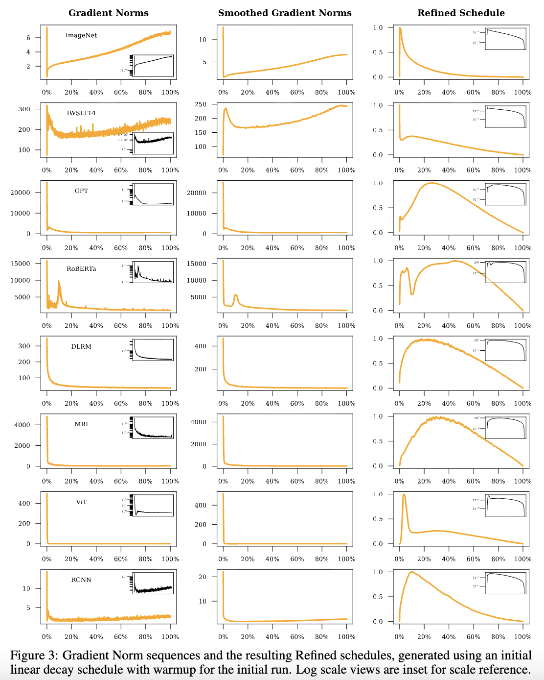
Some examples of Refined learning rates
Finally, the above results are for SGD, where $w_t\propto \mathbb{E}[\Vert\boldsymbol{g}(\boldsymbol{x}_t, \boldsymbol{\theta}_t)\Vert^{-2}]$. In practice, we can only use $\Vert\boldsymbol{g}(\boldsymbol{x}_t, \boldsymbol{\theta}_t)\Vert^2$ as an approximation, where $\Vert\cdot\Vert$ is the L2 norm. For adaptive learning rate optimizers like Adam, the paper suggests using $w_t\propto \mathbb{E}[\Vert\boldsymbol{g}(\boldsymbol{x}_t, \boldsymbol{\theta}_t)\Vert_1^{-1}]$, being inversely proportional to the L1 norm. We will discuss adaptive learning rate optimizers in later articles.
Explicit Version #
If we specify our own learning rate strategy $\eta_t$ and want to see how optimal it is, it currently seems quite troublesome because Eq. $\eqref{leq:last-6}$ is a semi-implicit conclusion. To substitute it into the right-hand side for verification, we must solve the equation $\eta_t = \frac{w_t w_{t+1:T}}{w_{1:T}}$. This equation isn't necessarily hard to solve, but the solution isn't elegant, making it difficult to use for a proof.
Here, through further scaling, we transform it into an explicit conclusion about $\eta_t$. The scaling requires some technique, which the author thought about for a long time, but it's easy to understand once written out: \begin{equation}\eta_t = \frac{w_t w_{t+1:T}}{w_{1:T}} \leq \frac{w_t (w_{t:T} + w_{t+1:T})}{2 w_{1:T}} = \frac{w_{t:T}^2 - w_{t+1:T}^2}{2 w_{1:T}}\end{equation} Here $w_{t:T}^2$ is understood as $(w_{t:T})^2$. Summing from $t \sim T$ on both sides: \begin{equation}\eta_{t:T} \leq \frac{w_{t:T}^2}{2 w_{1:T}}\end{equation} Substituting $t=1$ yields $\frac{1}{w_{1:T}} \leq \frac{1}{2\eta_{1:T}}$. Replacing $t$ with $t+1$ yields $\frac{w_{1:T}}{w_{t+1:T}^2} \leq \frac{1}{2\eta_{t+1:T}}$. Then combining this with the definition of $\eta_t$: $\frac{w_t^2}{w_{1:T}} = \eta_t^2 \frac{w_{1:T}}{w_{t+1:T}^2} \leq \frac{\eta_t^2}{2\eta_{t+1:T}}$. Finally, transforming the right side of Eq. $\eqref{leq:last-6}$ slightly and substituting these inequalities: \begin{equation}\mathbb{E}[L(\boldsymbol{\theta}_T) - L(\boldsymbol{\theta}^*)] \leq \frac{R^2}{2 w_{1:T}} + \sum_{t=1}^T \frac{w_t^2}{2 w_{1:T}} G_t^2 \leq \frac{R^2}{4 \eta_{1:T}} + \sum_{t=1}^{T-2} \frac{\eta_t^2}{4\eta_{t+1:T}} G_t^2 + \frac{w_{T-1}^2}{2 w_{1:T}} G_{T-1}^2 + \frac{w_T^2}{2 w_{1:T}} G_T^2 \end{equation} We did not scale the last two terms because, according to the definition $\eta_t = \frac{w_t w_{t+1:T}}{w_{1:T}}$, $\eta_T=0$ must hold, making $\frac{\eta_t^2}{2\eta_{t+1:T}}$ infinite at $t=T-1$ and $t=T$. This also tells us that $\eta_1,\eta_2,\cdots,\eta_T$ actually have only $T-1$ degrees of freedom, but the corresponding "unknowns" $w_1,w_2,\cdots,w_T$ contain $T$ variables. Since the number of equations is less than the number of unknowns, this provides a flexible degree of freedom for adjustment.
Following the definition, we have $\eta_{T-1} = \frac{w_{T-1} w_T}{w_{1:T}}$. Thus, from the AM-GM inequality: \begin{equation}\frac{w_{T-1}^2}{2 w_{1:T}} G_{T-1}^2 + \frac{w_T^2}{2 w_{1:T}}G_T^2 \geq \frac{w_{T-1} w_T}{w_{1:T}} G_{T-1}G_T = \eta_{T-1}G_{T-1}G_T \end{equation} Due to the existence of the "flexible degree of freedom," we can choose appropriate $w_{T-1}, w_T$ (specifically, by setting $w_{T-1} G_{T-1} = w_T G_T$) so that the above inequality reaches equality. Thus: \begin{equation}\mathbb{E}[L(\boldsymbol{\theta}_T) - L(\boldsymbol{\theta}^*)] \leq \frac{R^2}{4 \eta_{1:T}} + \sum_{t=1}^{T-2} \frac{\eta_t^2}{4\eta_{t+1:T}} G_t^2 + \eta_{T-1} G_{T-1} G_T\end{equation} The author hasn't seen this conclusion in any literature yet, so for now, it's considered new. Its precision is higher than $\eqref{leq:last-2}$. Of course, conclusion $\eqref{leq:last-2}$ isn't strictly applicable to learning rate sequences that end at zero, so a direct comparison is difficult, but looking at the constant coefficients of the first two main terms, Eq. $\eqref{leq:last-2}$ is $1/2$ while the formula above is $1/4$. On average, the precision should be doubled.
Summary #
At the end of the previous post, we mentioned the difficulty of proving the optimal learning rate strategy for terminal loss. In this article, through top-down, careful scaling and construction, we completed this proof and obtained a result with higher precision, while also discussing the enlightenment of this result on the "Warmup-Decay" mechanism of learning rates.